Deep reinforcement learning

This article aims to describe how to implement a Deep Reinforcement Learning (RL) using Approximation Q-Function with a Neural Network (NN) through an example of building a robot tank on the Robocode platform.

Source code: DeepQLearningRobot.

Approach

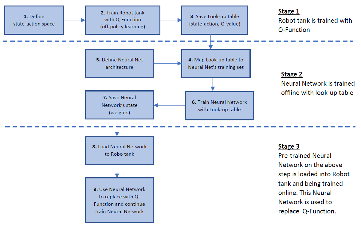
The implementation has three primary stages

1. Implement RL using tabular methods, e.g. Temporal-Difference learning (TD-learning).

   In particular, I use the simplest Q-Learning algorithm which is an extension of TD(0), in which the states, action, and appropriate Q-values are stored on a look-up table. This table is then saved for offline training on the next step.

2. Construct and train a NN using the saved look-up table above.

   I use a NN having multiple inputs as the state-action spaces and single output as the Q-value. I plan to improve the source code to support a different architecture that has multiple inputs and multiple outputs, in which the inputs are the states space while the outputs are the pairs of {action, Q-value}. I expect that it would reduce the computing time when exploring the best action based on the states space.

3. Implement Deep RL using Q-Function approximation with the pre-trained NN above.

   After having a RL implementation with Q-Learning algorithm, this step is a transision step to replace the look-up table with an approximate function which is a NN. The RL with Q-Function as a NN is also called Deep RL with Deep Q-Learning. The reason we should try to avoid using look-up table is that saving all state-action spaces requires a huge memory and data processing time, leading to be unrealistic for an environment that has a large state-action space.

The overall approach is shown in the image below.

Reinforcement Formulation

As RL is an algorithm to specify the appropriate Action of a specific States by learning from a Reward system, it is important to identify the following artifacts

• States
• Actions
• Reward

State

The state is captured by 3 sub-states

• State 1: the robot’s energy. It has 3 levels: low, medium, and high
• State 2: the distance from the robot to the enemy. It has 3 levels: veryClose, near and far
• State 3: the robot’s gun heat. It has 2 levels: low, high

Action

There are 4 following actions: Attack, Avoid, Runaway, Fire

Reward

• Bad terminal reward: reward - 10 if the robot is killed by the enemy.
• Good terminal reward: reward + 10 if the enemy is killed by the robot.
• Bad instant reward: reward -3 if the robot is hit by the enemy or wall.
• Good instant reward: reward + 3 if the robot hits the enemy.

Enemy

This Robot tank is trained and tested against the enemy Tracker. With the above formulation and using the Q-Learning algorithm, the robot has performed in 6000 rounds to save the latest (also the best) Look-up table to use for the next offline training step.

Offline training

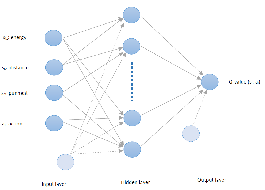
The neural network’s architecture used on this implementation has multiple inputs which is the state-action space vector and single output which is the corresponding Q-Value as illustrated in the image below

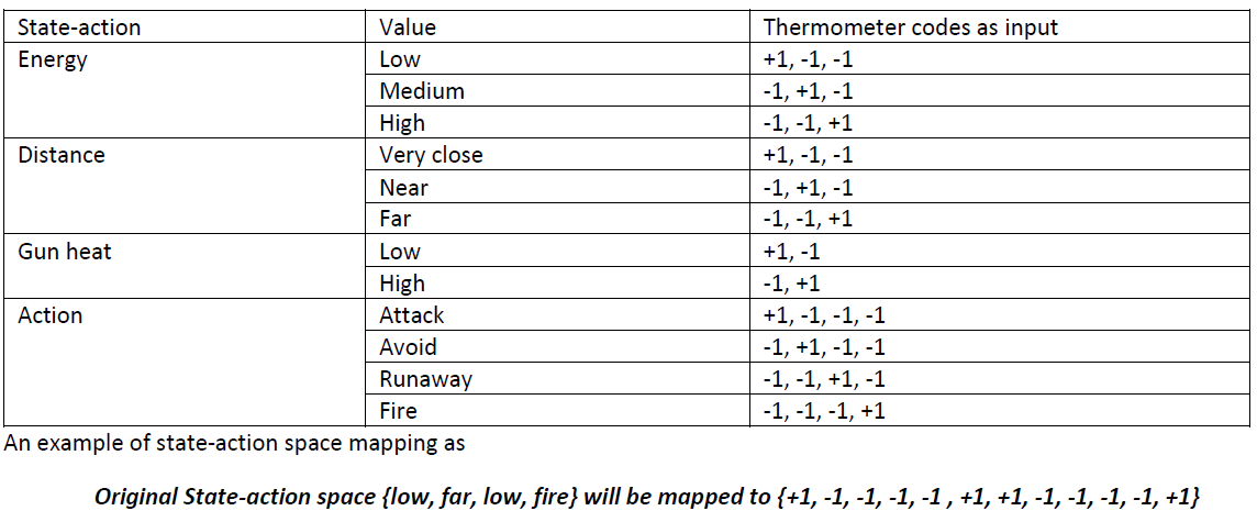
Input normalization

As all the state-action space values are continuous variables, the easiest way is to use “Thermometer” codes to present it. Using the same state-action space size, the mapping will look like image blow

Output normalization

The Q-value will also be normalized in the range [-1,1] to feed into the target output of the neural network. This can be done by scale the min/max Q-values to fall between [-1, 1]. Additionally, since there are few state-action spaces that are not visited, these Q-values will be over the normal range which should be considered as null data. Those values will be eliminated out of the training data set.

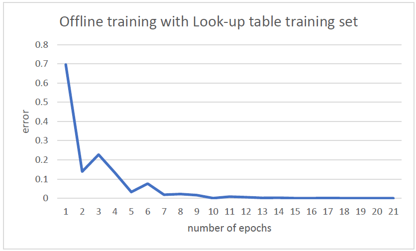
NN offline training

After having a set of inputs vectors and expected outputs, the neural network has been trained using backpropagation algorithm, and the best result is saved to be used for the online-training step - Number of Inputs: 12 (3 for Energy, 3 of Distance, 2 for GunHeat, and 4 for Action). - Number of Hidden Neurons: 12 - Learning Rate: 0.1 - Momentum: 0.9 - Activation function: bipolar sigmoid

Online training

Using the pre-trained neural network, the robot has continued online training with the Experiment Replay technique. The result of the neural network is shown in the image below.

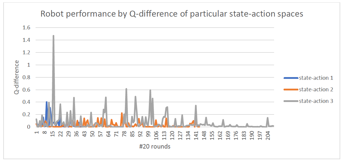
More details on how to implement Experiment Replay will be documented in another post later.

Setup

1. Setup Robocode environment with IntelliJ

   • Requirements
     • Oracle JDK 1.8
     • Robocode downloaded at robowiki
   • Pull this source code
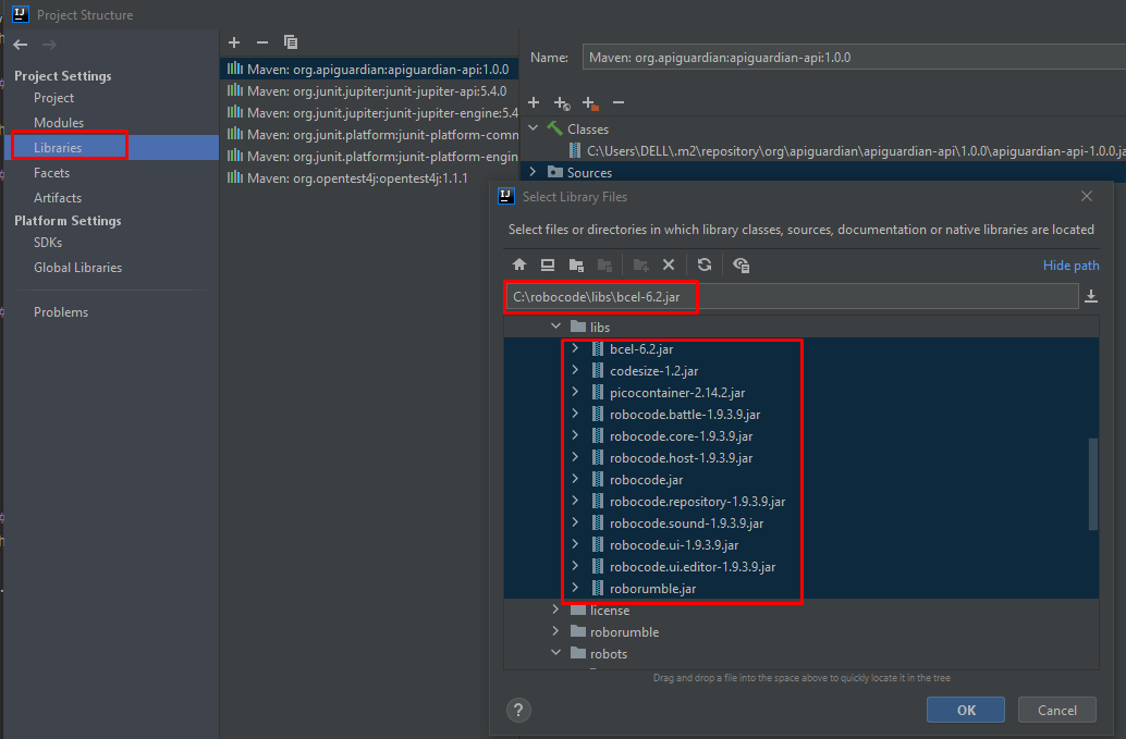
   • Add Robocode lib to project’s libs (image below)
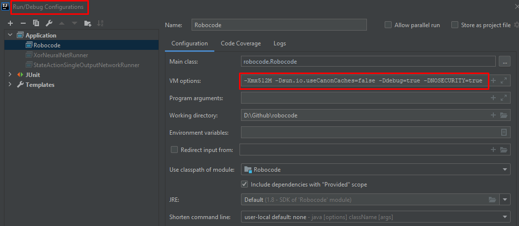
   • Create Robocode application and update its VM option (image below)
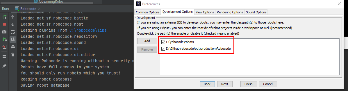
   • Run Robocode and add classes path folder to the “Development Options” (image below)
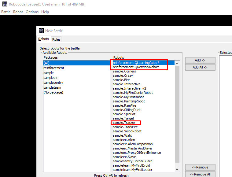
   • The two robots and robocode’s samples should be up and ready to fight. (image below)
   • Amend log and data folder on “\src\main\java\AppConfiguration”
2. Train QLearningRobo and save LUT table
   • Select QLearningRobo and Tracker for a battle in at least 6000 rounds.
   • The result is saved on the log folder, copy lut file to data folder with the name “lut.log”
3. Train the network and tune hyper-parameters with saved lut.log
   • Run “StateActionSingleOutputNetworkRunner” on “\test\java\backpropagation” with different hyper-parameters to find the best result
   • The result is saved on the log folder, copy the nn_weights.log file to the data folder
4. Train QNetworkRobo with saved nn_weights.log
   • Select QNetworkRobo and Tracker for another battle
   • The result is saved in the log folder

Related Articles

• How to train a neural network by using Backpropagation algorithm?