Backpropagation example with bipolar xor presentation

To have a better understanding how to apply backpropagation algorithm, this article is written to illustrate how to train a single hidden-layer using backpropagation algorithm with bipolar XOR presentation. It is just simply an example for my previous post about backpropagation neural network.

The neural nework architecture

The neural network using in this example has 2 inputs, 1 hidden layer with 4 neurons and 1 output, in which, the bipolar XOR training data set looks like below

Input X0	Input X1	Output Y
-1	-1	-1
-1	1	1
1	-1	1
1	1	-1

The neural network's architecture is illustrated in the following image

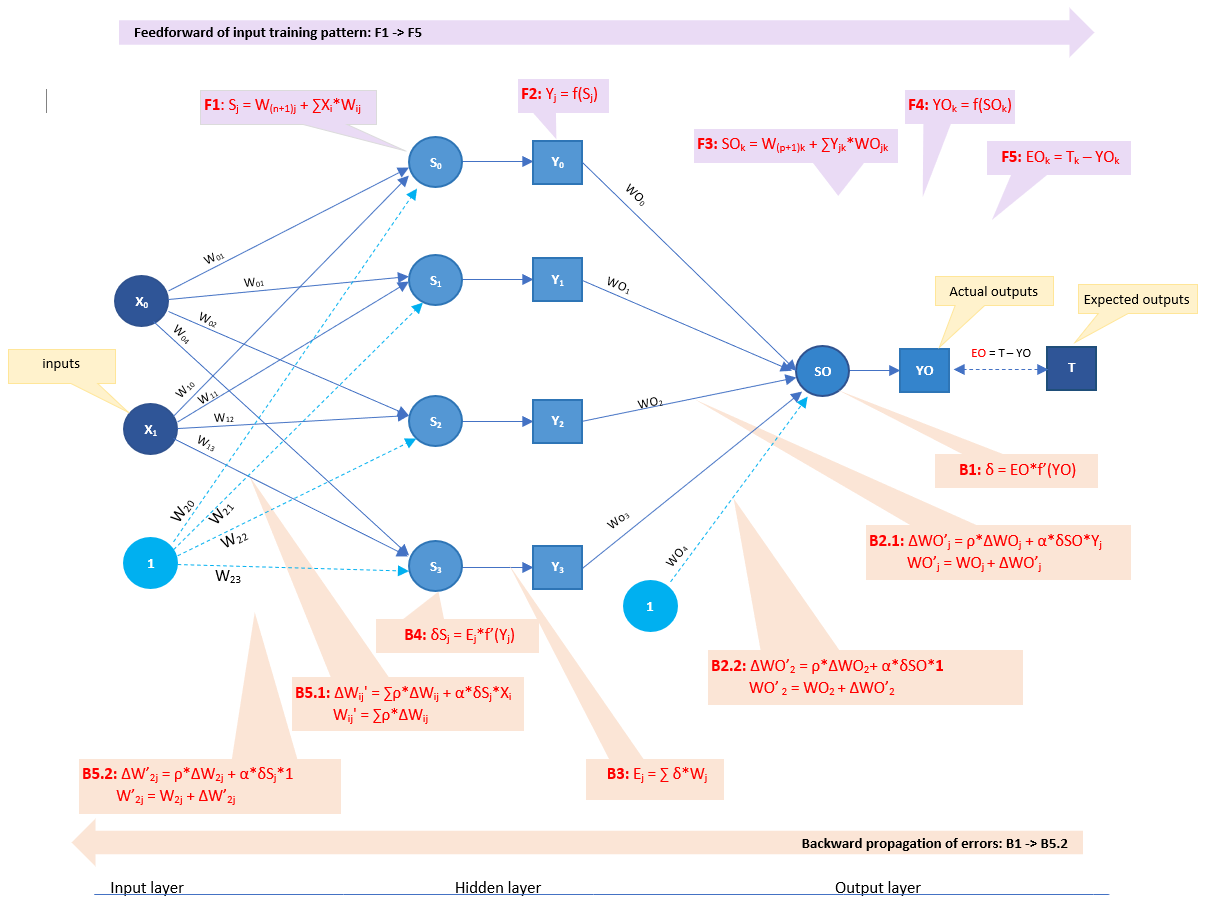
Figure 1: neural-network framework for XOR presentation

Error backpropagation algorithm

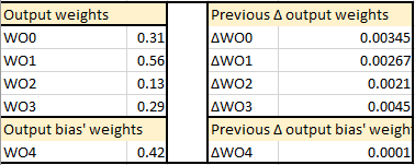
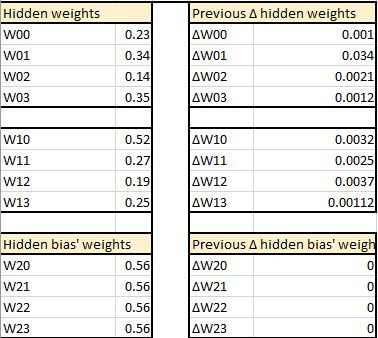
In this example, given a neural network with predefined hyper-parameters, weights, and delta weights, I will demonstrate how to perform step by step one full feedforward and backward propagation a specific pair of inputs {-1, -1}, and its expected output {-1} to adjust weights.

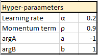
Neural network's predefined values

Predefined hyper-parameters

Predefined current weights and delta weights from hidden neurons and output bias to output

Predefined current weights and delta weights from inputs and hidden bias to hidden neurons

With given above values, it is ready to perform the feedforward round to compute error on the output as demonstrated on the next section.

Feedforward propagation

Using steps described on previous post about backpropagation neural network, I have following computations.
F1+F2: Input and output signals on each hidden neuron

F3+F4: Input and output signals on output

F5: Error on the output

Error = T - YO = -1.190506994

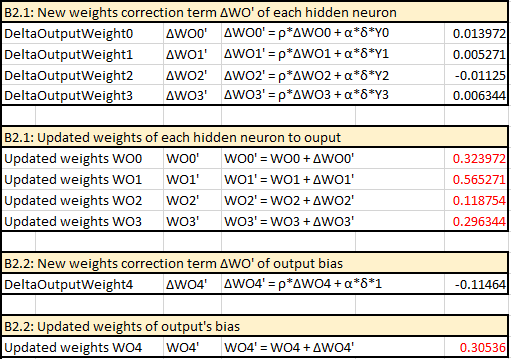
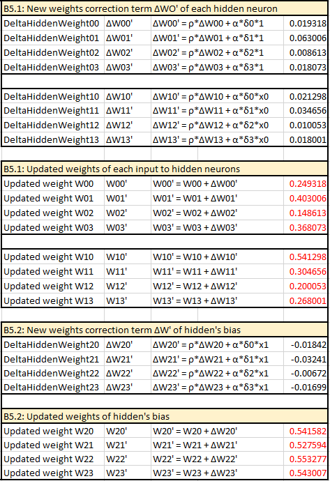
With the error found on the output, it will be backward propagated to adjust the weights, as demonstrated on the next section.

Error backward propagation

B1: Error signal term δ of output SO

B2.1 + B2.2: New weight correction terms and updated weights of each hidden neuron and output bias to the output

B3+B4: Given that the error at each hidden neuron is δ*WO_i, the error signal term δ of each hidden neuron is computed as below

B5.1 + B5.2: New weight correction terms and updated weights of each input and hidden bias to each hidden neuron

This procedure of the above feedforward and backward propagation will be repeated on each pair of inputs vector and its expected output. All the error found of each pattern will be summed up with the following formula to compute the final error of each iteration (aka, each epoch). \[ E = \frac{1}{2}*\sum_{k=0}^m (T_k - YO_k)^2 \] If this error is less than target error, this training is done. In other words, it reaches the convergence. Otherwise, the round of feedforward and error backward propagation will be repeated until it reaches the convergence or the number of iterations is over the limit, which is preconfigured as 20.000 on my implementation.

Data source:
If you feel interested, I am also glad to share how compute all the numbers above on this excel file

Fine-turning hyper-parameters tool

The XORNeuralNetRunner is written to test the XOR presentation's neural network in a number of trials until it reaches the limit or the convergence. This runner allows initializing different hyper-parameters for the neural-network as well as the target error of the training. On each test, the runner will perform a given number of trials, whereas on each trial, it will perform backpropagation to fine-tune the weights until it reach the target error or it reaches the limit of epochs. The hyper-parameters that are allowed to adjust are listed below

• Number of hidden neurons
• Activation-function used on hidden and output layers
• Target error
• Learning rate
• Momentum term
• Weights

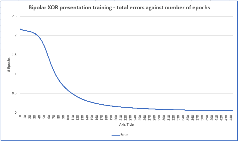
On each trial that reaches the convergence, it will save all the errors on every epoch to help draw a graph of total error against number of epochs as an example below