Backpropagation neural network

As part of my article about How to implement Deep Reinforcement Learning to build a robot tank?", this post is written to describe how the Backpropagation (BP) algorithm works since it will be used to implement the Function Approximation on the Deep Q-Learning. This article will only discuss the implementation aspects, so it is recommended to read the neural-network fundamentals in advance, e.g. the classical book "Fundamentals of Neural Networks" by Laurene Fausett.

Source code: backpropagation neural-network implementation.

Neural network architecture

This implementation supported the backpropagation algorithm for a single hidden layer neural-network, in which it has one multiple-input layer, one hidden layer with multiple neurons, and one multiple-output layer as illustrated on the following image. This architecture is adequate for a large number of applications.

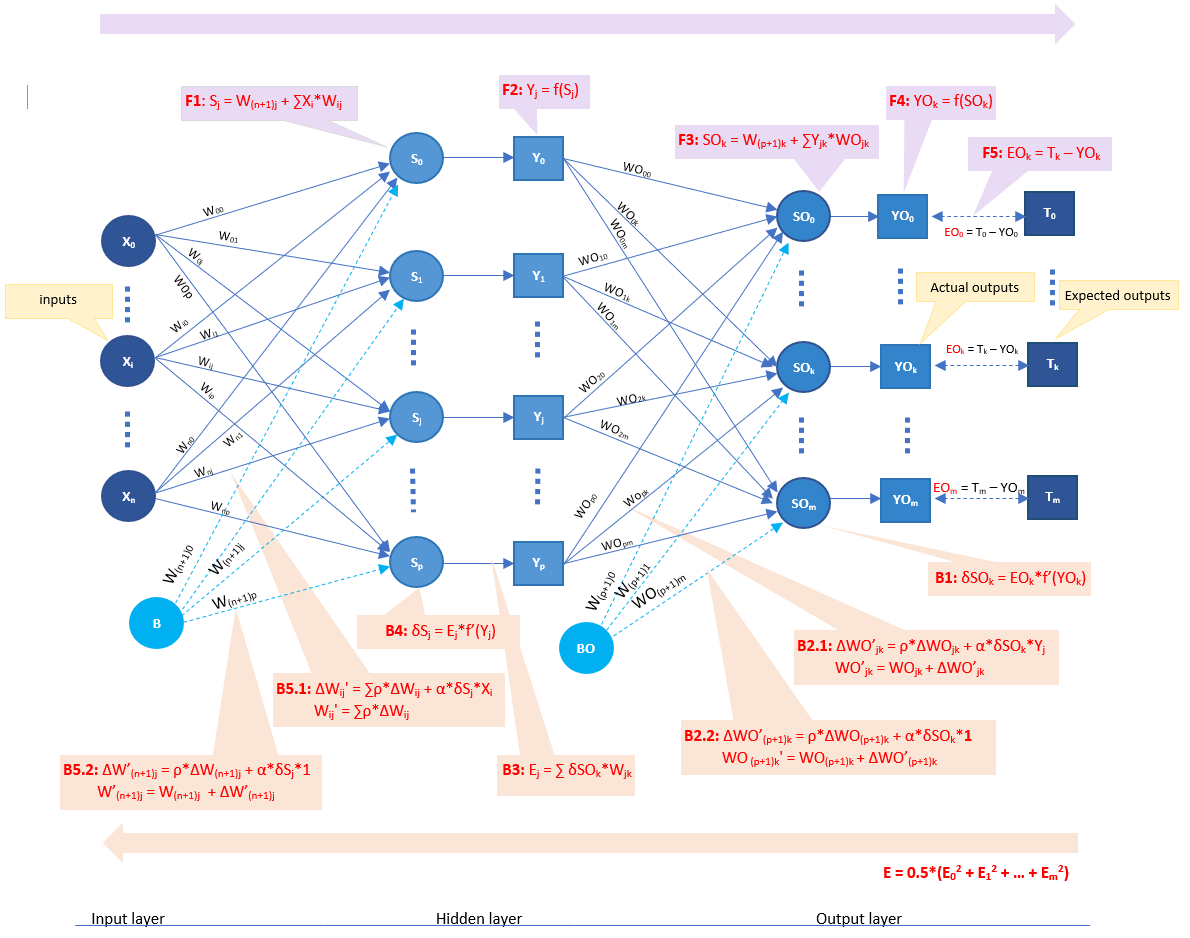
Figure 1: Single hidden layer neural-network framework

Bias vs weights

There is bias (value 1) on each hidden and output layer as depicted in the above image. The weights of those bias are variant and will also be adjusted during the training, just the same as how the other weights are updated during the training.

Activation function

The activation function used on each hidden layer and output layer can vary in each specific situation. I have supported 3 activation functions including TanH, Relu, Sigmoid. There is no evidence that we should use the same activation function for all layers, but for ease of implementation, I use the same activation function for all layers, and the default one is the generic binary or bipolar Sigmoid function.

Neural network's primary hyper-parameters

The neural-network is implemented in class "BackpropagationBaseNetwork.java" which is specified by following hyper-parameters

• Number of inputs: as in the above image, there are (n + 1) input training vectors from {X₀, ..., X_i to X_n.
• Number of hidden neurons: as in the above image, there are (p + 1) neurons on the hidden layer.
• Number of outputs: as in the above image, there are (m + 1) output target vectors from 0 {T₀, ..., T_i to T_m.
• Learning rate (α).
• Momentum tum (ρ): a variant of the stochastic gradient descent.
• argA: the lower pound of Sigmoid activation function used by both hidden and output layer.
• argB: the upper pound of Sigmoid activation function used by both hidden and output layer.

Notes
If the Sigmoid activation function is used (by default), we will have the activation function and derivative of the activation function as below \[ f(x) = \frac{(argB - argA)} {1+e^{-x} } + argA \] \[ f'(x) = \frac{1}{(argB - argA)} * (y - argA) * (argB - y) \]

Error Backpropagation algorithm

Error Backpropagation is the key and the most popular technique of training a neural network. This algorithm is simply a gradient descent method to fine-tune the weights by minimizing the total mean squared error (aka the loss) of the outputs computed by the network on each iteration (in the scope of this post, it is the same as each epoch).

A full training process for a neural-network is divided into 3 steps.

• Step 1: Initialize weights
• Step 2: for each pattern, perform training with the backpropagation algorithm
• Step 3: Recompute the loss (e.g. the root mean square, RMS). If it reaches the target error, then stop. Otherwise, turn back to step 2

Basically, training a network by backpropagation algorithm on each pattern on step 2 involves three stages

• Step 2.1: Perform feedforward of the inputs training pattern (inputs vector \(X_i\))
• Step 2.2: Perform backward propagation of the associated error (loss) on each output
• Step 2.3: Adjust the weights based on each computed error above

In the rest of this section, I will demonstrate how to perform all the above steps for a neural-network of n inputs, p hidden neurons, and m outputs. Additionally, the bias on the hidden layer is treated as another input with a value of 1, so there will be (n+1) inputs. Likewise, the bias on the output layer is put on as the hidden neuron (p+1).

Step 1: Initial weights

On my implementation, all weights are initialized with random values from [-0.5, 0.5].

Step 2.1: Feedforward propagation

The feedforward propagation is a process to compute the error (aka, the loss) on each output from an input vector. As illustrated in the above image, feedforward propagation has the following steps

• F1: For each inputs vector, calculate the value of each hidden neuron S_j by the following formula \[ S_j = W_(n+1)j + \sum_{i=0}^n W_{ij}*X_i \]
• F2: For each hidden neuron S_{j, apply the activation function to compute its output signal Yj by the following formula \[ Y_j = f(S_j) \]}
• F3: After getting output signals for all hidden neurons, calculate the value of each output neuron SO_k by the following formula \[ SO_k = W_(p+1)k + \sum_{j=0}^p W_{jk}*Y_k \]
• F4: For each output SO_k, apply the activation function to compute its output signal YO_k by the following formula \[ YO_k = f(SO_k) \]
• F5: Compute error EO_k (aka, loss) on each output by the following formula \[ EO_k = T_k - YO_k \]

Step 2.2 & 2.3: Backpropagation and weights update

The backpropagation is actually a process to propagate the error back to each hidden neuron to adjust the weights. As illustrated in the above image, backward propagation has the following steps

• B1: For each error EO_k, calculate the error signal term δ of SO_k by the following formula \[ δSO_k = EO_k*f'(YO_k) \]
• B2.1: For each error signal term δSO_k, calculate the new weights correction term ΔWO'_jk of that output SO_k to each hidden neuron Y_j by the following formula \[ ΔWO'_{jk} = ρ*ΔWO_{jk} + α*δSO_k*Y_j \] (Notice that, ΔWO'_jk is the new weight correction term which is derived from the error signal and a portion (momentum term ρ) of its previous weight correction term ΔWO_jk.)
  
  This delta ΔWO'_jk will be used to adjust the corresponding WO_jk, so the new weight is calculated by the following formula \[ WO'_{jk} = WO_{jk} + ΔWO'_{jk} \]
• B2.2: Similarly, calculate the new bias correction term ΔWO'_(p+1)k of that output SO_k to each hidden neuron Y_j by the following formula \[ ΔWO’_{(p+1)k} = ρ*ΔWO_{(p+1)k} + α*δSO_k*1 WO'_{(p+1)k} = WO_{(p+1)k} + ΔWO’_{(p+1)k} \]
• B3: After having all the weights to the output layer updated, calculate the new error at each hidden neuron E_j by the following formula \[ E_j = \sum_{k=0}^m W_{kj}*δSO_k \]
• B4: Calculate the error signal term δ of each hidden neuron S_j by the following formula \[ δS_j = E_j*f'(Y_j) \]
• B5.1: For each error signal term δS_j, calculate the new weights correction term ΔW'_ij of that neuron S_j to each input X_i by the following formula \[ ΔW'_{ij} = ρ*ΔW_{ij} + α*δS_j*X_i \] (Notice that, ΔW'_ij is the new weight correction term which is derived from the error signal and a portion (momentum term ρ) of its previous weight correction term ΔW_ij.)
  
  This delta ΔW'_ij will be used to adjust the corresponding W_ij, so the new weight is calculated by the following formula \[ W'_{ij} = W_{ij} + ΔW'_{ij} \]
• B5.2: Similarly, calculate the new bias correction term ΔW'_(n+1)j of that neuron S_j to each input X_i by the following formula \[ ΔW’_{(n+1)j} = ρ*ΔW_{(n+1)j} + α*δS_j*1 W'_{(n+1)j} = W_{(n+1)j} + ΔW’_{(n+1)j} \]

Step 3: Computed error of one inputs vector

There would be different approaches to compute the error corresponding to each input vector. On my implementation, I used the following formulation \[ E = \frac{1}{2}*\sum_{k=0}^m (T_k - YO_k)^2 \]

The training will be iterated until it reaches the convergence (aka, getting to target error) or until it is over the maximum number of iterations.

An example with XOR presentation
To elaborate the algorithm in practice, I demonstrated how it works with bipolar XOR presentation on the post an example of backpropagation with bipolar XOR presentation